Tutorial 4: Cascading Failures
Cascading failures often arise as a result of natural failures or targeted attacks in a network. Consider an electrical grid where a central substation goes offline. In order to maintain the distribution of power, neighboring substations have to increase production in order to meet demand. However, if this is not possible, the neighboring substation fails, which in turn causes additional neighboring substations to fail. The end result is a series of cascading failures i.e., a blackout. While cascading failures can occur in a variety of network types e.g., water, electrical, communication, we focus on the electrical grid. Below, we discuss the design and implementation of the cascading failure model and how TIGER can be used to both induce and prevent cascading failures using the attack and defense mechanisms discussed in previous tutorials. There are 3 main processes governing the network simulation:
capacity of each node \(c_v\in [0,1]\)
load of each node \(l_v\in U(0, l_{max})\)
network redundancy \(r\in [0, 1]\)
The capacity of each node \(c_v\) is the the maximum load a node can handle, which is set based on the node’s normalized betweenness centrality. The load of each node \(l_v\) represents the fraction of maximum capacity \(c_v\) that the node operates at. Load for each node \(c_v\) is set by uniformly drawing from \(U(0, l_{max})\), where \(l_{max}\) is the maximum initial load. Network redundancy r represents the amount of reserve capacity present in the network i.e., auxiliary support systems. At the beginning of the simulation, we allow the user to attack and defend the network according to the node attack and defense strategies discussed in previous tutorials. When a node is attacked it becomes “overloaded”, causing it to fail and requiring the load be distributed to its neighbors. When defending a node we increase it’s capacity to protect against attacks.
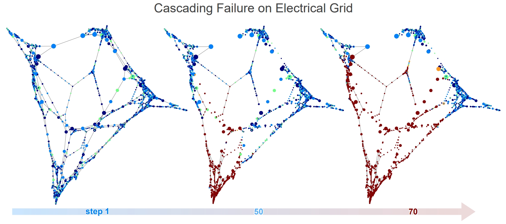
TIGER cascading failure simulation on the US power grid network when 4 nodes are overloaded according to the ID attack strategy. Time step 1: shows the network under normal conditions. Time step 50: we observe a series of failures originating from the bottom of the network. Time step 70: most of the network has collapsed.
To help users visualize cascading failures induced by targeted attacks, we enable them to create visuals like the figure above, where we overload 4 nodes selected by the ID attack strategy on the US power grid dataset (\(l_max=0.8\)). Nodesize represents capacity i.e., larger size \(\rightarrow\) higher capacity, and color indicates the load of each node on a gradient scale from blue (low load) to red (high load); dark red indicates node failure (overloaded). Time step 1 shows the network under normal conditions; at step 50 we observe a series of failures originating from the bottom of the network; by step 70 most of the network has collapsed.
To run a cascading failure simulations and create the visual, we just have to write a few lines of code:
from graph_tiger.cascading import Cascading
from graph_tiger.graphs import graph_loader

graph = graph_loader('electrical')

params = {
   'runs': 1,
   'steps': 100,
   'seed': 1,

   'l': 0.8,
   'r': 0.2,
   'c': int(0.1 * len(graph)),

   'k_a': 30,
   'attack': 'rb_node',
   'attack_approx': int(0.1 * len(graph)),

   'k_d': 0,
   'defense': None,

   'robust_measure': 'largest_connected_component',

   'plot_transition': True,  # False turns off key simulation image "snapshots"
   'gif_animation': False,  # True creaets a video of the simulation (MP4 file)
   'gif_snaps': False,  # True saves each frame of the simulation as an image

   'edge_style': 'bundled',
   'node_style': 'force_atlas',
   'fa_iter': 2000,
}

cascading = Cascading(graph, **params)
results = cascading.run_simulation()

cascading.plot_results(results)
We can also summarize simulation results over many configurations, and create plots the figure below, which shows the effect of network redundancy when 4 nodes are overloaded by the ID attack strategy. At 50% redundancy, we observe a critical threshold where the network is able to redistribute the increased load. For \(r < 50%\), the cascading failure can be delayed but not prevented.
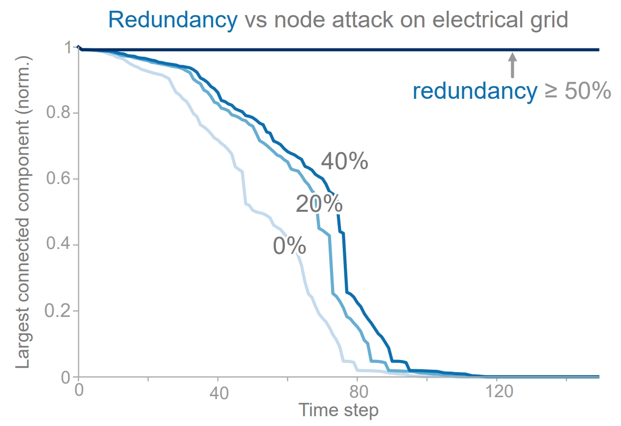
Effect of network redundancy r on the US power grid where 4 nodes are overloaded using ID. When \(r\geq 50\%\) the network is able to redistribute the increased load.
Running and visualizing multiple simulations only takes a few extra lines of code:
params = {
     'runs': 10,
     'steps': 100,
     'seed': 1,

     'l': 0.8,
     'r': 0.2,
     'c': int(0.1 * len(graph)),

     'k_a': 5,
     'attack': 'id_node',
     'attack_approx': None,  # int(0.1 * len(graph)),

     'k_d': 0,
     'defense': None,

     'robust_measure': 'largest_connected_component',

     'plot_transition': False,
     'gif_animation': False,

     'edge_style': None,
     'node_style': 'spectral',
     'fa_iter': 2000,

 }

 results = defaultdict(list)
 redundancy = np.arange(0, 0.5, .1)

 for idx, r in enumerate(redundancy):
     params['r'] = r

     if idx == 2:
         params['plot_transition'] = True
         params['gif_animation'] = True
         params['gif_snaps'] = True
     else:
         params['plot_transition'] = False
         params['gif_animation'] = False
         params['gif_snaps'] = False

     cf = Cascading(graph, **params)
     results[r] = cf.run_simulation()

 plot_results(graph, params, results, xlabel='Steps', line_label='Redundancy', experiment='redundancy')
def plot_results(graph, params, results, xlabel='Steps', line_label='', experiment=''):
   plt.figure(figsize=(6.4, 4.8))

   title = '{}:step={},l={},r={},k_a={},attack={},k_d={},defense={}'.format(experiment, params['steps'], params['l'], params['r'], params['k_a'],
                                                                                 params['attack'], params['k_d'], params['defense'])
   for strength, result in results.items():
      result_norm = [r / len(graph) for r in result]
      plt.plot(result_norm, label="{}: {}".format(line_label, strength))

   plt.xlabel(xlabel)
   plt.ylabel(params['robust_measure'])
   plt.ylim(0, 1)

   save_dir = os.getcwd() + '/plots/' + experiment + '/'
   os.makedirs(save_dir, exist_ok=True)

   plt.legend()
   plt.title(title)
   plt.savefig(save_dir + title + '.pdf')
   plt.show()
   plt.clf()