Tutorial 1: Measuring Vulnerability and Robustness

Robustness is defined as a measure of a network’s ability to continue functioning when part of the network is naturally damaged or targeted for attack :cite`ellens2013graph,chan2016optimizing,beygelzimer2005improving`. TIGER contains numerous robustness measures, grouped into one of three categories depending on whether the measure uses the graph, adjacency, or Laplacian matrix. In the figure below, we show some common robustness measures from each category.

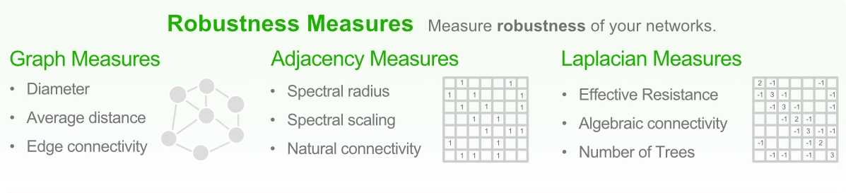
Robustness measures fall into one of three categories, depending on whether it uses the graph, adjacency, or Laplacian matrix.

Comparing Robustness Measures

We select 3 robustness measures, one from each of the above categories, to extensively discuss.

1. Average vertex betweenness (\(\bar{b}_v\)) of a graph \(G=(V, E)\) is the summation of vertex betweenness \(b_u\) for every node \(u \in V\), where vertex betweenness for node u is defined as the number of shortest paths that pass through u out of the total possible shortest paths

\[\begin{split}\bar{b}_v = \sum_{u\in V}\sum_{s\in V}\sum_{\substack{t\in V \\ s\neq t\neq u}} \frac{n_{s,t}(u)}{n_{s,t}}\end{split}\]

where \(n_{s, t}(u)\) is the number of shortest paths betweeen s and t that pass through t and \(n_{s, t}\) is the total number of shortest paths between s and t. Average vertex betweenness has a natural connection to graph robustness since it measures the average load on vertices in the network. The smaller the average the more robust the network, since load is more evenly distributed across nodes. In order to calculate this for measure for a graph, you can simply run the following:

from graph_tiger.measures import run_measure
from graph_tiger.graphs import graph_loader

graph = graph_loader(graph_type='BA', n=1000, seed=1)

avg_vertex_betweenness = run_measure(graph, measure='average_vertex_betweenness')
print("Average vertex betweenness:", avg_vertex_betweenness)

Since calculting the average vertex betweenness for large graphs is not computationally feasible, we can find a “close” approximate version by running the following code

from graph_tiger.measures import run_measure
from graph_tiger.graphs import graph_loader

graph = graph_loader(graph_type='BA', n=1000, seed=1)

avg_vertex_betweenness = run_measure(graph, measure='average_vertex_betweenness_approx', k=10)
print("Approximate average vertex betweenness:", avg_vertex_betweenness)

Since we are using an approximate version, the results will differ slightly from the full version. However, the advantage is that approximate versions can scale much better to large graphs. Selecting variable k is method dependent, however, we set reasonable default values for each method. We’ll do an in-depth comparison on how to practically set k at the end of the tutorial.

2. Spectral scaling (\(\xi\)) indicates if a network is simultaneously sparse and highly connected, known as “good expansion” (GE). Intuitively, we can think of a network with GE as a network lacking bridges or bottlenecks. In order to determine if a network has GE, the spectral gap is combined with odd subgraph centrality \(SC_{odd}\), which measures the number of odd length closed walks a node participates in. Formally, spectral scaling is described as

\[\xi(G) = \sqrt{\frac{1}{n} \sum_{i=1}^{n} \{log[\textbf{u}_1(i)] - [log\textbf{A} + \frac{1}{2} log[SC_{odd}(i)]] \}^2 }\]

where \(\textbf{A} = [sinh(\lambda_1)]^{-0.5}, n\) is the number of nodes, and \(\textbf{u}_1\) is the first eigenvector of adjacency matrix A. The closer \(\xi\) is to zero, the better the expansion properties and the more robust the network. Formally, a network is considered to have GE if \(\xi < 10^{-2}\), the correlation coefficient \(r < 0.999\) and the slope is 0.5.

3. Effective resistance (\(R\)) views a graph as an electrical circuit where an edge \((i, j)\) corresponds to a resister of \(r_{ij} = 1\) Ohm and a node i corresponds to a junction. As such, the effective resistance between two vertices i and j, denoted \(R_{ij}\), is the electrical resistance measured across i and j when calculated using Kirchoff’s circuit laws. Extending this to the whole graph, we say the effective graph resistance R is the sum of resistances for all distinct pairs of vertices. Klein and Randic proved this can be calculated based on the sum of the inverse non-zero Laplacian eigenvalues:

\[R = \frac{1}{2}\sum_{i, j}^{n} R_{ij} = n\sum_{i=2}^{n} \frac{1}{\mu_i}\]

As a robustness measure, effective resistance measures how well connected a network is, where a smaller value indicates a more robust network. In addition, the effective resistance has many desirable properties, including the fact that it strictly decreases when adding edges, and takes into account both the number of paths between node pairs and their length.

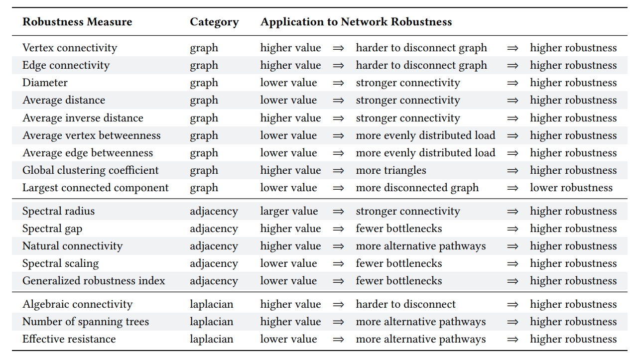
Comparison of TIGER robustness measures. Measures are grouped based on whether they use the graph, adjacency or Laplacian matrix. For each measure, we briefly describe it’s application to measuring network robustness.

Approximate vs Non-Approximate

Below, we’ll implement 5 robustness measures, and their approximate counterparts, so we can see how approximation value k affects the measurement quality. We can think of parameter k as representing the trade-off between speed (low k) and precision (high k).

import os
import numpy as np
from tqdm import tqdm
import matplotlib.pyplot as plt

if __name__ == '__main__':

   # compare 2 measures based on graph connectivity
   measures_graph = [
     'average_vertex_betweenness',
     'average_edge_betweenness',
     'average_vertex_betweenness_approx',
     'average_edge_betweenness_approx'
   ]

   # compare 3 measures based on graph Laplacian matrix
   measures_spectral = [
     'natural_connectivity',
     'number_spanning_trees',
     'effective_resistance',
     'natural_connectivity_approx',
     'number_spanning_trees_approx',
     'effective_resistance_approx',
   ]

   # graph params
   n = 300  # number of graph nodes
   start = 5  # k = 5
   step = 10  # k += 10

   # spectral params
   n_s = 300  # number of graph nodes
   start_s = 5  # k = 5
   step_s = 10  # k += 10

In this code block, we are just setting up the measures to compare and their associated parameters. Next, we are going to run each of the methods across different values of k to gather some data.

# run the graph measures, averaging the results over 30 randomly generated graphs
graph_results = run_analysis(n=n, runs=30, k_start=start, k_step=step, measures=measures_graph)

x_data = list(range(start, n, step)) + [300]
plot_results(x_data, graph_results, "graph", measures_graph, n, start, step)


# run the spectral measures, averaging the results over 30 randomly generated graphs
spectral_results = run_analysis(n=n_s, runs=30, k_start=start_s, k_step=step_s, measures=measures_spectral)

x_data_s = list(range(start_s, n_s, step_s)) + [300]
plot_results(x_data_s, spectral_results, "spectral", measures_spectral, n, start_s, step_s)

In order to run each robustness measure, do the following:

def run_analysis(n, runs, k_start, k_step, measures):
   from graph_tiger.graphs import graph_loader

   graphs = [graph_loader(graph_type='CSF', n=n, seed=s) for s in range(runs)]  # generate 30 random `clustered scale free` graphs

   approx_results = []
   k_values = list(range(k_start, n, k_step)) + [np.inf]
   for k in tqdm(k_values):
      results = []
      for i in range(runs):
         r = run(graphs[i], measures, k=k)
         results.append(r)

      k_avg = np.mean(results, axis=0)
      approx_results.append(k_avg)

   return np.stack(approx_results)



def run(graph, measures, k):
   result = []

   for measure in measures:
      if '_approx' in measure:
         measure = measure.replace('_approx', '')
         r = run_measure(graph=graph, measure=measure, k=k)
      else:
         r = run_measure(graph=graph, measure=measure)

      result.append(r)

   return result

Now that we have the results for all 5 measures at different values of k, along with non-approximate results (k=np.inf), we can plot the error between the non-approximate and the approximate robustness measure as a function of k.

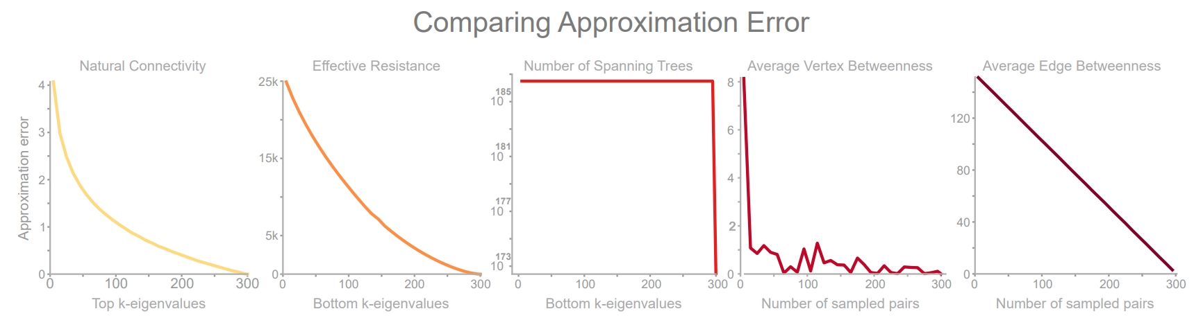
Error of 5 fast, approximate robustness measures supported by TIGER. Parameter k represents the trade-off between speed (low k) and precision (high k). To measure approximation efficacy, we vary \(r\in [5, 300]\) in increments of 10 and measure the error between the approximate and original measure averaged over 30 runs on a clustered scale-free graph with 300 nodes.

def plot_results(x_data, results, result_type, measures, n, start, step):
   num_measures = int(len(measures) / 2)
   fig, axes = plt.subplots(ncols=num_measures, figsize=(num_measures*6 - 1, 5))

   for index, metric_name in enumerate(measures):
      if index == num_measures:
         break

      error = np.round(np.abs(results[:, num_measures + index] - results[:, index]), 2)
      axes[index].plot(x_data, error, label=metric_name)

      axes[index].set_title(metric_name)
      axes[index].set_xlabel('k')
      axes[index].set_ylabel('Error')

      if metric_name == 'number_spanning_trees':
         axes[index].set_yscale('log')

  plt.legend(loc="upper right")

  save_dir = os.getcwd() + '/plots/'
  os.makedirs(save_dir, exist_ok=True)
  plt.savefig(save_dir + 'approximation_{}_n={},start={},step={}.pdf'.format(result_type, n, start, step))
  plt.show()