Introduction

TIGER is a Python Toolbox for evaluatIing Graph vulnErability and Robustness. TIGER contains numerous state-of-the-art methods to help users conduct graph vulnerability and robustness analysis on graph structured data. Specifically, TIGER helps users:

• Quantify network vulnerability and robustness.

• Simulate a variety of network attacks, cascading failures and spread of dissemination of entities.

• Augment a network’s structure to resist attacks and recover from failure.

• Regulate the dissemination of entities on a network (e.g., viruses, propaganda).

For additional information, take a look at our paper:

Evaluating Graph Vulnerability and Robustness using TIGER. Freitas, Scott, and Chau, Duen Horng. arXiv, 2020.

Background & Motivation

First mentioned as early as the 1970’s, network robustness has a rich and diverse history spanning numerous fields of engineering and science. This diversity of research has generated a variety of unique perspectives, providing fresh insight into challenging problems while equipping researchers with fundamental knowledge for their investigations. While the fields of study are diverse, they are linked by a common definition of robustness, which is defined as a measure of a network’s ability to continue functioning when part of the network is naturally damaged or targeted for attack.

The study of network robustness is critical to the understanding of complex interconnected systems. For example, consider an example of a power grid network that is susceptible to both natural failures and targeted attacks. A natural failure occurs when a single power substation fails due to erosion of parts or natural disasters. However, when one substation fails, additional load is routed to alternative substations, potentially causing a series of cascading failures. Not all failures originate from natural causes, some come from targeted attacks, such as enemy states hacking into the grid to sabotage key equipment to maximally damage the operations of the electrical grid. A natural counterpart to network robustness is vulnerability, defined as measure of a network’s susceptibility to the dissemination of entities across the network, such as how quickly a virus spreads across a computer network.

Unfortunately, the nature of cross-disciplinary research also comes with significant challenges. Oftentimes important discoveries made in one field are not quickly disseminated, leading to missed innovation opportunities. We believe a unified and easy-to-use software framework is key to standardizing the study of network robustness, helping accelerate reproducible research and dissemination of ideas.

Installation

To quickly get started, install TIGER using pip:

pip install graph-tiger

Alternatively, you can git clone TIGER and create a new Anaconda environment using the provided YAML file.

Citing

@article{freitas2020evaluating,
          title = {Evaluating Graph Vulnerability and Robustness using TIGER},
          author = {Freitas, Scott and Chau, Duen Horng},
          journal={arXiv preprint arXiv:2006.05648},
          year = {2020},
 }

Examples

We provide detailed tutorials on how to user TIGER in the Tutorials section. Below we look at a few simple examples to quickly get you started.

Example 1: Measuring graph robustness

How to measure graph robustness using the spectral methods: measures.spectral_radius() and measures.effective_resistance().

from graph_tiger.measures import run_measure
from graph_tiger.graphs import graph_loader

graph = graph_loader(graph_type='BA', n=1000, seed=1)

spectral_radius = run_measure(graph, measure='spectral_radius')
print("Spectral radius:", spectral_radius)

effective_resistance = run_measure(graph, measure='effective_resistance')
print("Effective resistance:", effective_resistance)

Example 2: Measuring approximate graph robustness

How to measure approximate graph robustness using spectral method: measures.effective_resistance().

from graph_tiger.measures import run_measure
from graph_tiger.graphs import graph_loader

graph = graph_loader(graph_type='BA', n=1000, seed=1)

effective_resistance = run_measure(graph, measure='effective_resistance', k=30)
print("Effective resistance (k=30):", effective_resistance)

Example 3: Cascading Failure Simulation

In this example, we run a cascading failure simulation on a Barabasi Albert (BA) graph. In the network, node size represents load capacity (i.e., larger size -> higher capacity), and color indicates the load of each node on a gradient scale from blue (low load) to red (high load); dark red indicates node failure (overloaded). Below, we show a TIGER cascading failure simulation on a BA graph when 30 nodes in the network randomly fail (untargeted attack).

from graph_tiger.cascading import Cascading
from graph_tiger.graphs import graph_loader

graph = graph_loader('BA', n=400, seed=1)

params = {
    'runs': 1,
    'steps': 100,
    'seed': 1,

    'l': 0.8,
    'r': 0.2,
    'c': int(0.1 * len(graph)),

    'k_a': 30,
    'attack': 'rb_node',
    'attack_approx': int(0.1 * len(graph)),

    'k_d': 0,
    'defense': None,

    'robust_measure': 'largest_connected_component',

    'plot_transition': True,  # False turns off key simulation image "snapshots"
    'gif_animation': False,  # True creaets a video of the simulation (MP4 file)
    'gif_snaps': False,  # True saves each frame of the simulation as an image

    'edge_style': 'bundled',
    'node_style': 'force_atlas',
    'fa_iter': 2000,
}

cascading = Cascading(graph, **params)
results = cascading.run_simulation()

cascading.plot_results(results)

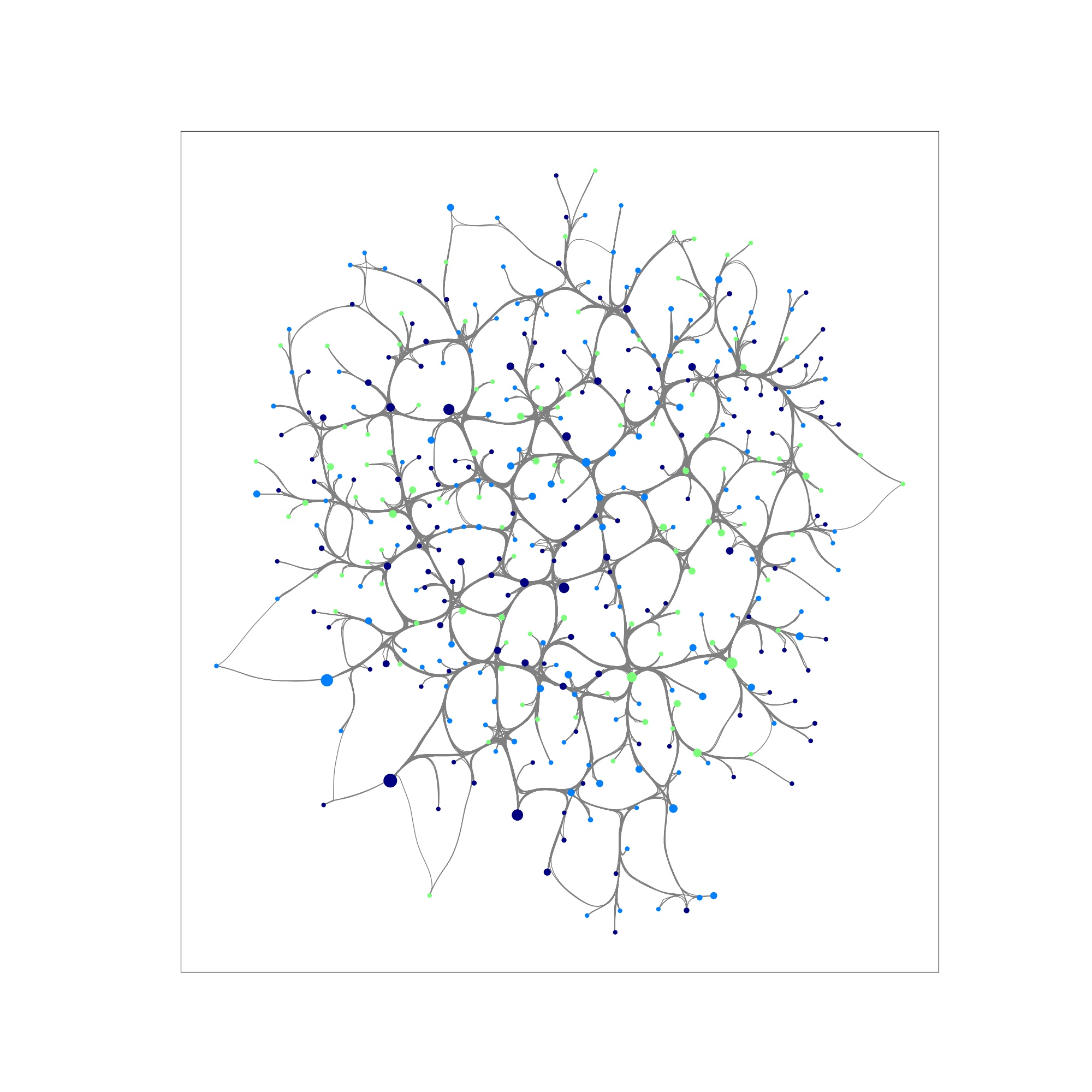
Time step 0: shows the network under normal operating conditions.

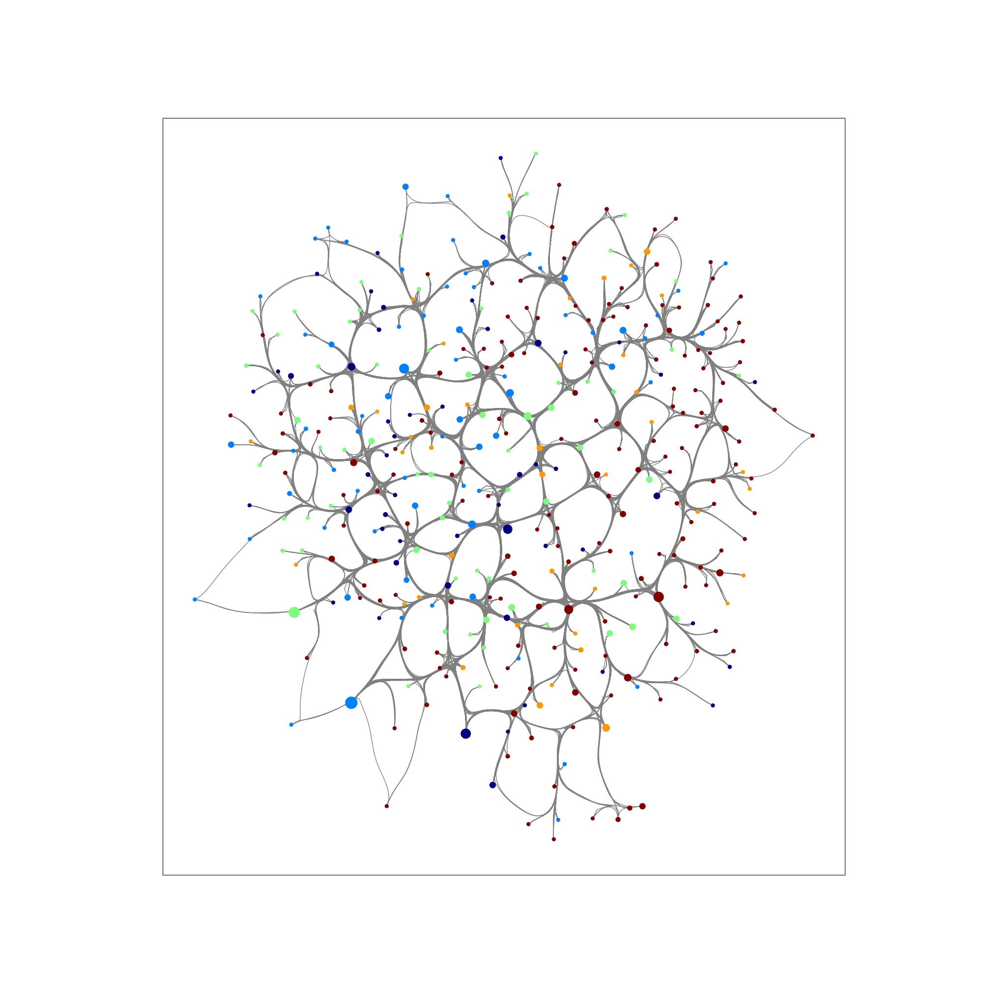
Step 5: we observe a series of failures across the network.

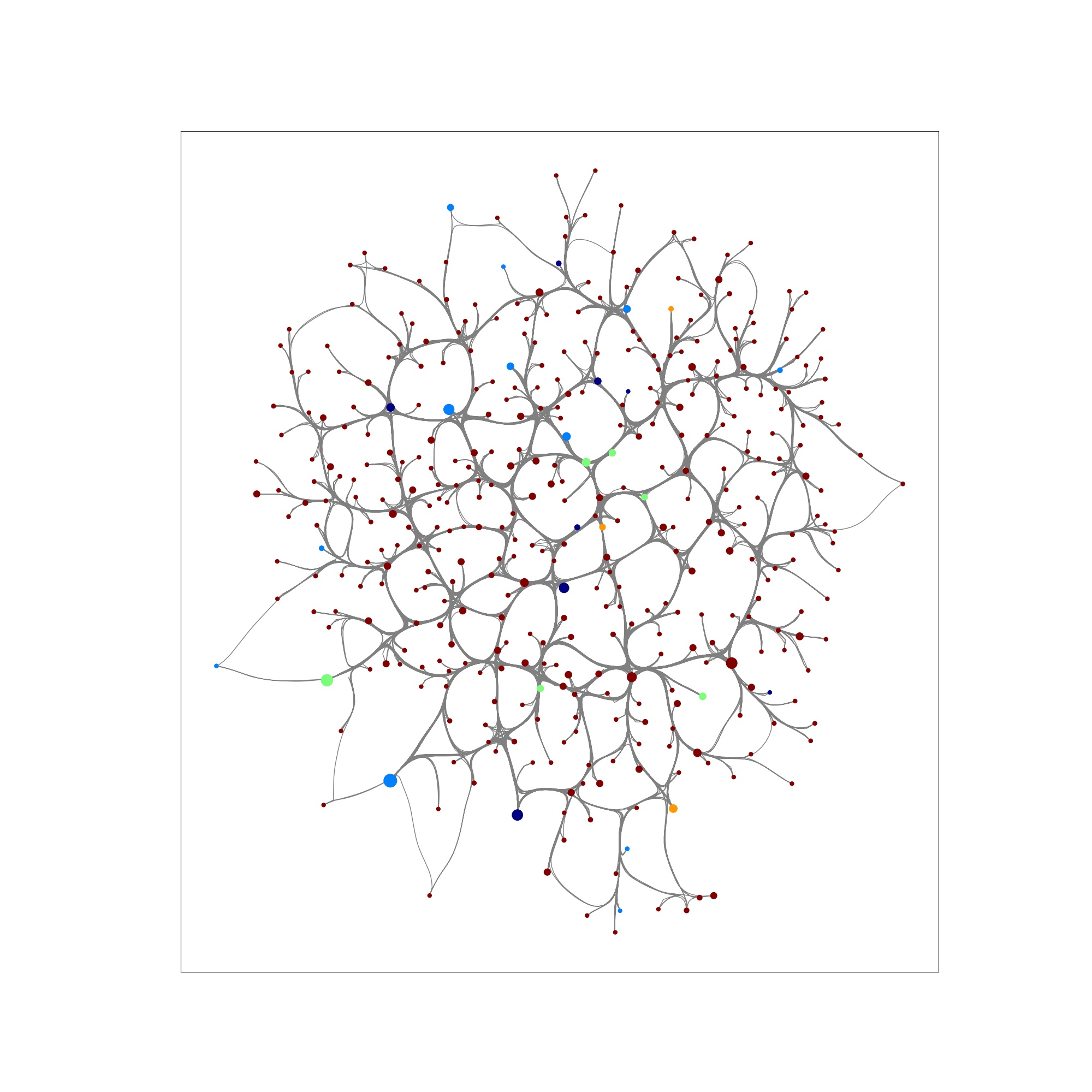
Step 99: most of the network has collapsed.

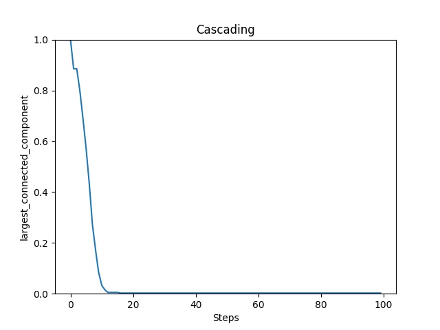
Graph connectivity over time (measured by graph’s largest connected component) during attack.

Example 4: SIS Model Network Vaccination

In this example, we run a computer virus simulation (SIS infection model) on a BA graph. The network starts off highly infected, and the goal is to vaccinate critical nodes to reduce disease resurgence. Using the Netshield techniqe, we select 5 nodes to vaccinate to maximally reduce the infection.

from graph_tiger.diffusion import Diffusion
from graph_tiger.graphs import graph_loader

graph = graph_loader('BA', n=400, seed=1)

sis_params = {
    'model': 'SIS',
    'b': 0.001,
    'd': 0.01,
    'c': 1,

    'runs': 1,
    'steps': 5000,
    'seed': 1,

    'diffusion': 'min',
    'method': 'ns_node',
    'k': 5,

    'plot_transition': True,
    'gif_animation': False,

    'edge_style': 'bundled',
    'node_style': 'force_atlas',
    'fa_iter': 2000
}

diffusion = Diffusion(graph, **sis_params)
results = diffusion.run_simulation()

diffusion.plot_results(results)

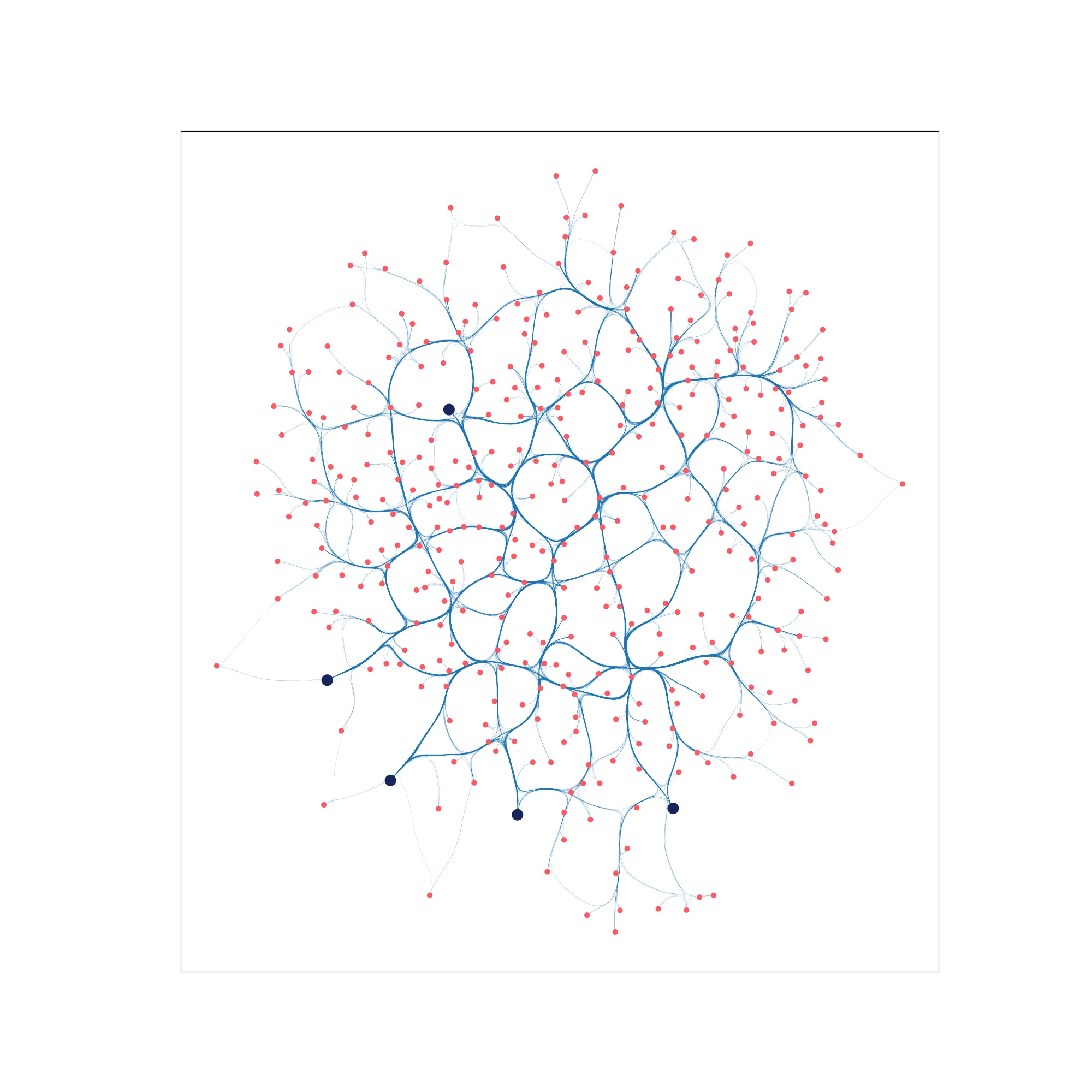
Step 0: A highly infected network with 4 nodes “vaccinated” according to Netshield defense.

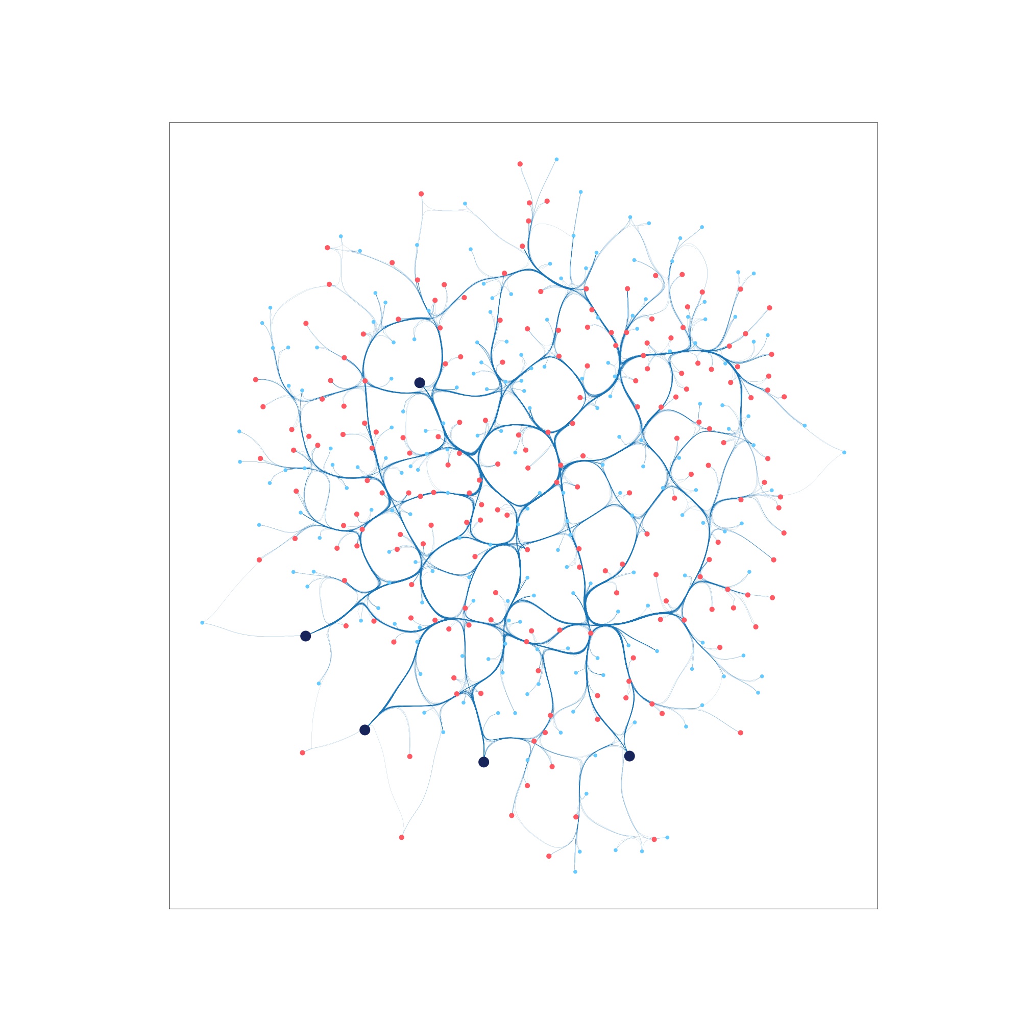
Step 80: The computer virus begins to remit.

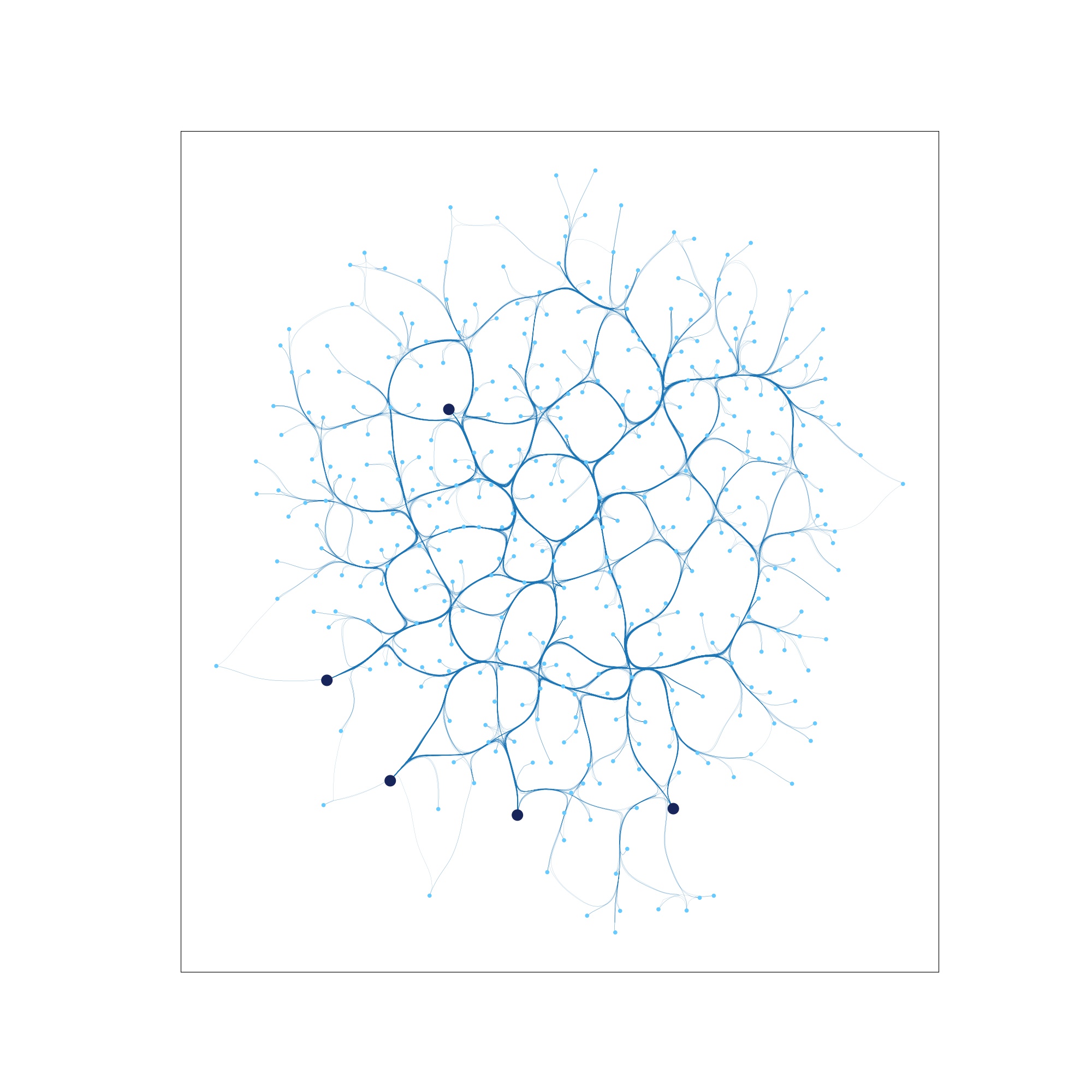
Step 4999: The virus is nearly contained.

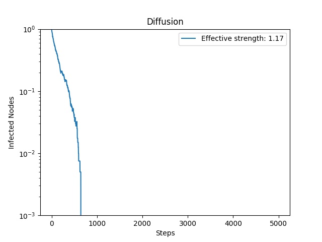
A plot of the number of infected nodes in the network at each time stamp.

Note

Figures will auto-populate in the “plots” folder.