Tutorial 2: Attacking a Network

There are two primary ways a network can become damaged: (1) natural failure and (2) targeted attack. Natural failures typically occur when a piece of equipment breaks down from natural causes. In the study of graphs, this would correspond to the removal of a node or edge in the graph. While random network failures regularly occur, they are typically less severe than targeted attacks. In contrast, targeted attacks carefully select nodes and edges in the network for removal in order to maximally disrupt network functionality. As such, we focus the majority of our attention to targeted attacks.

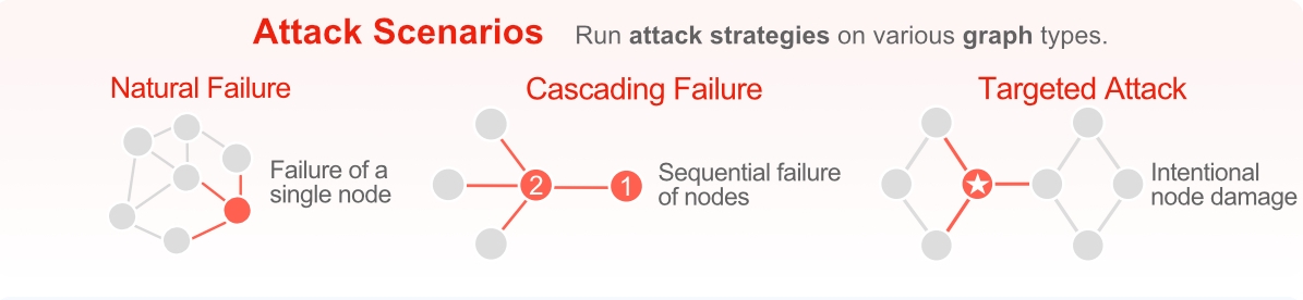
Networks can become damaged through natural failures or targeted attacks. Depending on the severity of the damage, networks can suffer from cascading failures.

We showcase an example attack in the figure below on the Kentucky KY-2 water distribution network. The network starts under normal conditions (far left), and at each step an additional node is removed by the attacker (red nodes). After removing only 13 of the 814 nodes, the network is split into two separate regions. By step 27, the network splits into four disconnected regions. In this simulation, and in general, attack strategies rely on node and edge centrality measures to identify candidates. If we look carefully, we observe that certain nodes (and edges) in the network act as key bridges between various network regions. As a result, attacks able to identify these bridges are highly effective in disrupting this network. Below, we discuss several attack strategies contained in TIGER and then compare their effectiveness on attacking the Kentucky KY-2 water distribution network.

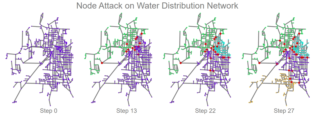
TIGER simulation of an RD node attack on the KY-2 water distribution network. Step 0: network starts under normal conditions; at each step a node is removed by the attacker (red nodes). Step 13, 22 & 27: after removing only a few of the 814 nodes, the network splits into two and three and four disconnected regions, respectively.

• Initial degree removal (ID) targets nodes with the highest degree \($\delta_v\). This has the effect of reducing the total number of edges in the network as fast as possible. Since this attack only considers its neighbors when making a decision, it is considered a local attack. The benefit of this locality is low computational overhead.

• Initial betweenness removal (IB) targets nodes with high betweenness centrality \(b_v\). This has the effect of destroying as many paths as possible. Since path information is aggregated from across the network, this is considered a global attack strategy. Unfortunately, global information comes with significant computational overhead compared to a local attacks.

• Recalculated degree (RD) and betweenness removal (RB) follow the same process as ID and IB, respectively, with one additional step to recalculate the degree (or betweenness) distribution after a node is removed. This recalculation often results in a stronger attack, however, recalculating these distributions adds a significant amount of computational overhead to the attack.

In the figure below, we can see the effectiveness of each attack strategy when used to remove nodes and edges from a network, where attack success is measured based on how fractured the network becomes when removing nodes from the network (i.e., largest connected component). We identify three key observations: (i) random node removal (RND) is not an effective strategy on this network structure; (ii) RB is the most effective attack strategy; and (iii) the remaining three attacks are roughly equivalent, falling somewhere between RND and RB. Now lets take a look at how to implement this in code using TIGER. We begin by setting up the attack parameters and creating an attack visualization on the Kentucky KY-2 water distribution network.

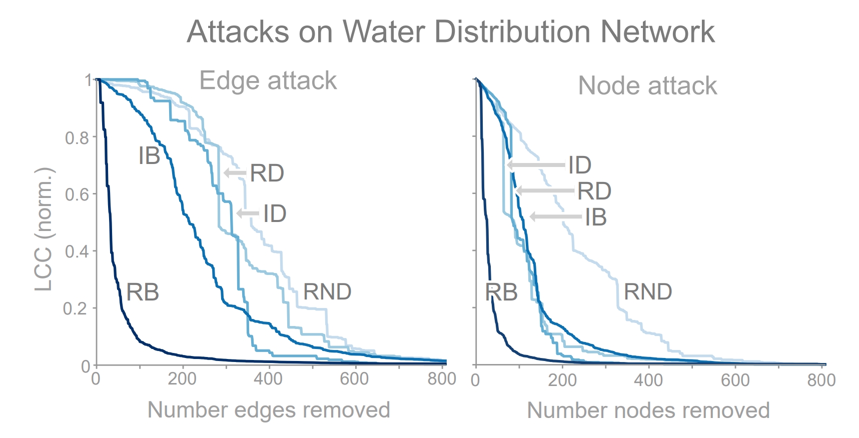
Efficacy of 5 edge attacks (left) and 5 node attacks (right) on the KY-2 water distribution network. The most effective attack (RB) disconnects approximately 50% of the network with less than 30 removed edges (or nodes).

import os
import sys
import matplotlib.pyplot as plt
from collections import defaultdict

from graph_tiger.attacks import Attack
from graph_tiger.graphs import graph_loader

graph = graph_loader(graph_type='ky2', seed=1)

params = {
     'runs': 1,
     'steps': 30,
     'seed': 1,

     'attack': 'rb_node',
     'attack_approx': int(0.1*len(graph)),

     'plot_transition': True,
     'gif_animation': True,
     'gif_snaps': True,

     'edge_style': None,
     'node_style': None,
     'fa_iter': 20
 }

 print("Creating example visualization")
 a = Attack(graph, **params)
 a.run_simulation()

Next, we want to test the effectiveness of a variety of node-based attacks on the water network. In addition, we average the results over multiple runs to obtain representative results.

 params['runs'] = 10
 params['steps'] = len(graph) - 1
 params['plot_transition'] = False
 params['gif_animation'] = False
 params['gif_snaps'] = False

 print("Running node attacks")
 results = defaultdict(str)
 for attack in node_attacks:
     params['attack'] = attack

     if 'rb' in attack or 'ib' in attack:
         params['attack_approx'] = int(0.1*len(graph))
     else:
         params['attack_approx'] = None

     a = Attack(graph, **params)
     results[attack] = a.run_simulation()
 plot_results(graph, params['steps'], results, title='water:node-attacks_runs={}'.format(params['runs']))

Now we repeat the attacks to identify critical edges, instead of attack network nodes.

 print("Running edge attacks")
 results = defaultdict(str)
 for attack in edge_attacks:
     params['attack'] = attack

     if 'rb' in attack or 'ib' in attack:
         params['attack_approx'] = int(0.1*len(graph))
     else:
         params['attack_approx'] = None

     a = Attack(graph, **params)
     results[attack] = a.run_simulation()
 plot_results(graph, params['steps'], results, title='water:edge-attacks_runs={}'.format(params['runs']))

Finally, we use this helper function to make all of the plots.

def plot_results(graph, steps, results, title):
   plt.figure(figsize=(6.4, 4.8))

   for method, result in results.items():
      result = [r / len(graph) for r in result]
      plt.plot(list(range(steps)), result, label=method)

   plt.ylim(0, 1)
   plt.ylabel('LCC')
   plt.xlabel('N_rm / N')
   plt.title(title)
   plt.legend()

   save_dir = os.getcwd() + '/plots/'
   os.makedirs(save_dir, exist_ok=True)

   plt.savefig(save_dir + title + '.pdf')
   plt.show()
   plt.clf()